May 16, 2008
The Helpful Undergraduate: Another Response to James Annan
In his latest essay on my stupidity, climate modeler James Annan made the helpful suggestion that I consult a “a numerate undergraduate to explain it to [me].” So I looked outside my office, where things are quiet out on the quad this time of year, but as luck would have it, I did find a young lady named Megan, who just happened to be majoring in mathematics who agreed to help me overcome my considerable ignorance.
The first thing I had to do was explain to Megan the problem we are looking at. I told her that we had 55 estimates of a particular quantity, with a mean of 0.19 and standard deviation of 0.21. At the same time we had 5 different observations of that same quantity, with a mean of –0.07 and standard deviation of 0.07. I wanted to know how similar or different from each other these two sets of data actually were.
I explained to her that James Annan, a modest, constructive, and respectful colleague of mine who happened to be a climate modeler (“Cool” she said), had explained that the best way to compare these datasets was to look at the normal distribution associated with the data (N(0.19. 0.21) and plot on that distribution the outlying value from the smaller dataset.
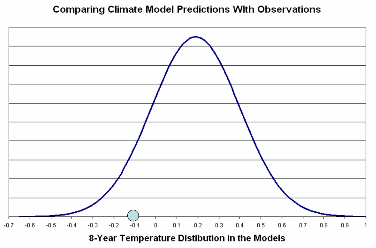
Since the outlying value of the observations fell well within the distribution of the estimates, James told us, the two dataset could not be claimed to be different — case closed, anyone saying anything different must be an ignorant climate denying lunatic.
“Professor Pielke,” Megan said, “You are funny. James surely didn’t react that way, because since he is a climate modeler he must surely recognize that there are many ways to look at statistical problems. We even learned that just this year in our intro stats class. Besides, I can’t imagine a scientific colleague being so rude! You must have misinterpreted him.”
Since Megan was being so helpful in my education, I simply replied that we should stick to the stats. Besides, if she really knew that I was a climate denying moron, she might not continue to help me.
Megan said, “There is another way to approach this problem. Have you heard of an unpaired t-test for two different samples? (PDF)”
I replied, “Of course not, I am just a political scientist.”
Megan said, “We learned in stats this year that such a test is appropriate for comparing two distributions with equal variance to see how similar they are. It is really very easy. In fact you can run these tests online using a simple calculator. Here is one such website that will do all of the work for you, just plug in the numbers.”
So we plugged our numbers into the magic website as follows:
Sample 1:
Mean = 0.19
SD = 0.21
N = 55
Sample 2
Mean = -0.07
SD = 0.07
N = 5
And here is what the magic website reported back:
Unpaired t test results
P value and statistical significance:
The two-tailed P value equals 0.0082
By conventional criteria, this difference is considered to be very statistically significant.
Confidence interval:
The mean of Group One minus Group Two equals -0.2600
95% confidence interval of this difference: From -0.4502 to -0.0698Intermediate values used in calculations:
t = 2.7358
df = 58
standard error of difference = 0.095
“Wow,” I said to Megan, “These are lots of numbers. What do they all mean?”
“Well,” Megan helpfully replied, “They mean that there is a really good chance that your two distributions are inconsistent with each other.”
“But,” I protested, “Climate modeler James Annan came up with a different result! And he said that his method was the one true way!”
“You are kidding me again, Professor Pielke,” she calmly replied, “Dr. Annan surely recognizes that there are a lot of interesting nuances in statistical testing and using and working with information. There are even issues that can be raised about the appropriateness of test that we performed. So I wouldn’t even be too assured that these results are the one true way either. But they do indicate that there are different ways to approach scientific questions. I am sure that Dr. Annan recognizes this, after all he is a climate scientist. But we’ll have to discuss those nuances later. I’m taking philosophy of science in the fall, and would be glad to tutor you in that subject as well. But for now I have to run, I am on summer break after all.”
And just like that she was gone. Well, after this experience I am just happy that I was instructed to find a smart undergraduate to help me out.
[UPDATE An alert reader notes this comment by Tom C over at James' blog, which is right on the mark:
James -
What you and Roger are arguing about is not worth arguing about. What is worth arguing about is the philosophy behind comparing real-world data to model predictions. I work in the chemical industry. If my boss asked me to model a process, I would not come back with an ensemble of models, some of which predict an increase in a byproduct, some of which predict a decrease, and then claim that the observed concentration of byproduct was "consistent with models". That is just bizarre reasoning, but, of course, such a strategy allows for perpetual CYAing.
The fallacy here is that you are taking models, which are inherently different from one another, pretending that they are multiple measurements of a variable that differ only due to random fluctuations, then doing conventional statistics on the "distribution". This is all conceptually flawed.
Moreover, the wider the divergence of model results, the better the chance of "consistency" with real-world observations. That fact alone should signal the conceptual problem with the approach assumed in your argument with Roger.
Another commenter tries to help out James by responding to Tom C, but in the process, also hits the nail on the head:
I don't see what the problem is, Tom C. It seems obvious that the less specific a set of predictions is, the more difficult it is to invalidate. So yes, consistency doesn't neccessarily mean that your model is meaningful, especially over such short terms.
Right! "Consistent with" is not a meaningful statement. Which is of course where all of this started.
[UPDATE #2]
The figure below shows the IPCC distribution of 55 forecasts N[0.19, 0.21] as the blue curve, and I have invented a new distribution (red curve) by adding a bunch of hypothetical nonsense forecasts such that the distribution is now N[0.19, 1.0].
The blue point represents a hypothetical observation.
According to the metric of evaluating forecasts and observations proposed by James Annan my forecasting ability improved immensely simply by adding 55 nonsense forecasts, since th blue observational point now falls closer to the center of the new (and improved distribution).
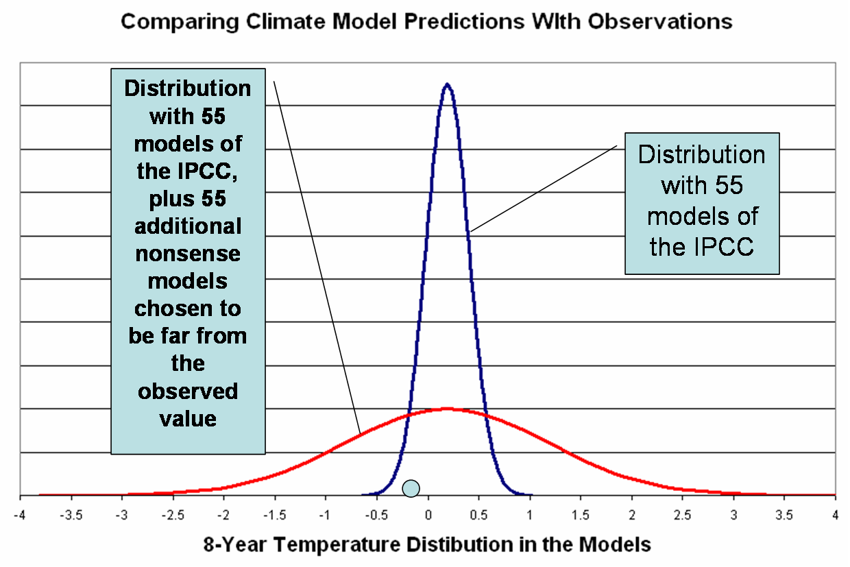
Now if James wants to call this an improvement (“more consistent whit” — “higher statistical significance” — etc.], but any approach that lends greater consistency by making adding worse forecasts to your distributions fails the common sense test.
[UPDATE #3]
Real Climate says this about a model-observation comparison in a recent paper by Knutson et al. in Nature Geoscience on hurricanes:
The fact that the RCM-based downscaling approach can reproduce the observed changes when fed modern reanalysis data is used by Knutson et al as a ‘validation’ of the modeling approach (in a very rough sense of the word–there is in fact a non-trivial 40% discrepancy in the modeled and observed trends in TC frequency). But this does not indicate that the downscaled GCM projections will provide a realistic description of future TCs in combination with a multi-model GCM ensemble mean. It only tells us that the RCM can potentially provide a realistic description of TC behavior provided the correct input.
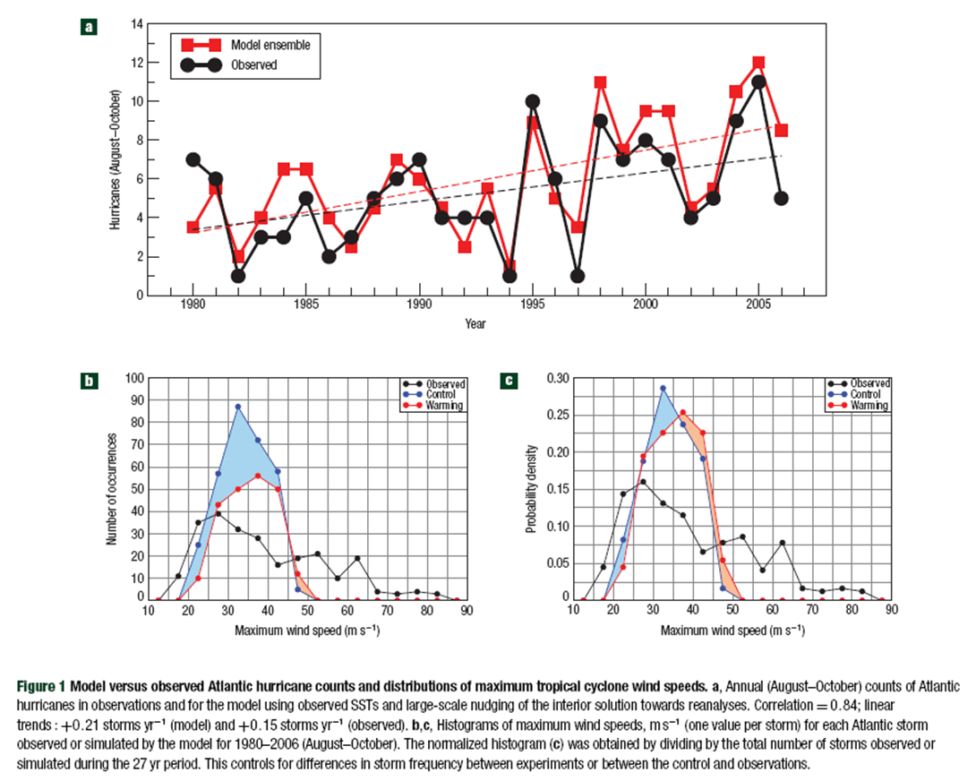
Have a look at the figure below, and the distributions of modeled and observations. Its funny how the differences in these distributions is considered to be “non-trivial” but the larger differences in temperature trends is “not inconsistent with” model predictions. Further proof of the irrelevance of the notion of “consistency.”