May 29, 2006
Evaluating Jim Hansen’s 1988 Climate Forecast
A lot of attention has been paid by both sides of the climate debate to a prediction made in 1988 before Congress by NASA scientist James Hansen. Today this forecast is the subject of an op-ed by Paul Krugman in the New York Times in which he accuses a prominent climate skeptic of scientific fraud. For some time I have been interested in various claims about Jim Hansen’s forecast because I am interested in prediction and its use/misuse in policy and politics. But what has been missing to date is a rigorous evaluation of Hansen’s forecast. Here is an initial effort to bring a bit more rigor to such an evaluation. The numbers below are not the last word, may contain errors, and are intended to open a discussion on this subject.
Hansen’s 1988 prediction was based on an analysis presented in this paper:
Hansen, J., I. Fung, A. Lacis, D. Rind, S. Lebedeff, R. Ruedy, G. Russell, and P. Stone 1988. Global climate changes as forecast by Goddard Institute for Space Studies three-dimensional model. J. Geophys. Res. 93, 9341-9364. (Abstract)
The paper generated future climate predictions based on three scenarios, described in the abstract as follows:
Scenario A assumes continued exponential trace gas growth, scenario B assumes a reduced linear linear growth of trace gases, and scenario C assumes a rapid curtailment of trace gas emissions such that the net climate forcing ceases to increase after the year 2000.
In this PDF, Jim Hansen provided an image of the prediction for the three scenarios with an overlay of the actual temperature increase in a response to Michael Crichton. I have reproduced the figure immediately below.
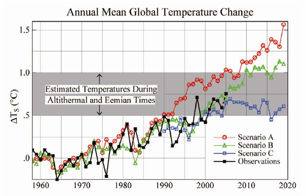
The observations (black) are very closely matched to Scenario B. Consequently, Jim Hansen claimed, “the real world has followed a course closest to that of Scenario B” (PDF). But is this correct? It appears that Jim Hansen may have gotten the right answer on temperature for the wrong reasons because his assumptions about emissions paths were not accurate. Further, Scenario B with the best match to temperature is the most inaccurate with respect to emissions projections.
The three scenarios used by Jim Hansen were based on assumptions about how society would produce emissions forward from 1988. Key assumptions were made for methane (CH4), Nitrous Oxide (N2O), and Carbon Dioxide (CO2) – For scenarios A and B in developing and developed countries, and for the global total in the case of Scenario C. Here are the assumptions from Hansen’s 1988 paper for growth rates in CH4, N2O, and CO2:
Scenario A
CH4 0.5%
N2O 0.25%
CO2 3% developing, 1% developed
Scenario B
CH4 0.25%
N2O 0.25%
CO2 2% developing, 0% developed
Scenario C
CH4 0.0%
N2O 0.25%
CO2 1.6 ppm increase annually
In order to evaluate whether these assumptions played out as projected in the three scenarios I consulted online databases with estimates of increases in CH4, N2O, and CO2.
I found CH4 data for 1990-2005 in an EPA report (PDF) in Appendix A-II.
I found N2O data for 1990-2005 in the same EPA report (PDF) in Appendix A-3.
I found CO2 data from the UN FCCC in a recent report (PDF) , for Annex I countries in table II-3 for 1990-2003.
I found global CO2 levels for 1990-2005 in the U.S. government database.
I used this data to compare growth rates in CH4, N2O, and CO2 to Jim Hansen’s 3 scenarios from 1988. Here is what I found:
Actual Rate of Increase
CH4 0.46%
N2O 0.95%
CO2 -0.52% (Annex 1 Countries 1990-2003)
CO2 >4.5% (Non-Annex 1 Countries 1990-2003)
CO2 1.5 PPM (1990-2005)
Comparison with Scenarios
Most Accurate CH4 Assumption = Scenario A
Most Accurate N2O Assumption = each
Most Accurate CO2 Assumption = Scenario C
In none of the three emissions assumptions did Scenario B contain the most accurate emissions assumptions. From this initial evaluation, it seems that to the extent that Jim Hansen’s Scenario B has accurately anticipated global temperature increases since 1988, it has done so based on inaccurate assumptions about emissions paths. Perhaps the errors cancel out, but an accurate prediction based on inaccurate assumptions should give some pause to using those same assumptions into the future. I am not sure which Scenario would be evaluated as the most accurate, but given the importance of CO2 as a greenhouse gas, I’d lean toward Scenario C. None of this is to doubt that global temperature has increased or will continue to increase as projected by the IPCC.
The usual caveats apply: This analysis provides no support for anyone who would cherry pick one scenario over another to evaluate their accuracy (as Paul Krugman has accused Patrick Michaels and Michael Crichton of doing). Nor does this analysis provide any reason not to support the importance of action on climate policy.
What it does, however, is raise questions about how scientists are treated differently in the public by other scientists and the media, and importantly, how some instances of policy-relevant science are framed critically and other instances are framed quite positively. Take William Gray for example who spent decades warning about a coming increase in hurricane activity, who was proven correct when activity increased, only to be frequently excoriated by his peers for his views on global warming. On hurricanes, Gray may have been right for the wrong reasons, but he was nonetheless right in his warning. Hansen on the other hand, is feted by his peers and the media yet just like Bill Gray may have been right for the wrong reasons.